lecture03_example – CBE 20260

# ==============================================================================
# LECTURE 3: Forms of Energy and Calculating Work
# Script: Maxwell-Boltzmann Demo
# Author: Edward Maginn, CBE 20260
# Description: 
#   This notebook lets you interactively explore the Maxwell–Boltzmann speed distribution
#   and connect it to molecular kinetic energy.

# Learning goals
# - See how the distribution **shifts and broadens** as temperature increases
# - Compare how **molecular mass** changes the typical speeds
# - Verify numerically that  
#  $[\left\langle \tfrac{1}{2} m v^2 \right\rangle = \tfrac{3}{2} k_B T]$

# Tip: Run cells top-to-bottom once. Then use the sliders/dropdowns to explore.
# ==============================================================================

import numpy as np
import math
import matplotlib.pyplot as plt

# Interactive widgets (works in JupyterLab/Notebook; in some environments you may need:
#   pip install ipywidgets
#   jupyter nbextension enable --py widgetsnbextension

import ipywidgets as widgets
from IPython.display import display, Markdown

# Physical constants
kB = 1.380649e-23  # Boltzmann constant, J/K
NA = 6.02214076e23 # Avogadro's number, 1/mol
R  = 8.314462618   # Gas constant, J/(mol K)

# A small library of molecules (molar mass in g/mol)
species_db = {
    "Helium (He)": 4.0026,
    "Hydrogen (H2)": 2.01588,
    "Nitrogen (N2)": 28.0134,
    "Oxygen (O2)": 31.9988,
    "Carbon dioxide (CO2)": 44.0095,
    "Water vapor (H2O)": 18.01528,
    "Argon (Ar)": 39.948,
}

# Functions to calculate
def molar_mass_to_molecule_mass(M_g_per_mol: float) -> float:
    """Convert molar mass (g/mol) to mass per molecule (kg)."""
    return (M_g_per_mol * 1e-3) / NA

def f_MB(v: np.ndarray, m: float, T: float) -> np.ndarray:
    """Maxwell–Boltzmann speed distribution f(v) for speeds v (m/s)."""
    pref = 4 * math.pi * (m / (2 * math.pi * kB * T))**(1.5)
    return pref * v**2 * np.exp(-(m * v**2) / (2 * kB * T))

def speeds_characteristic(m: float, T: float):
    """Most probable, mean, and RMS speeds."""
    v_mp = math.sqrt(2 * kB * T / m)
    v_mean = math.sqrt(8 * kB * T / (math.pi * m))
    v_rms = math.sqrt(3 * kB * T / m)
    return v_mp, v_mean, v_rms

display(Markdown("✅ **Setup complete.** Use the interactive cell below."))

✅ Setup complete. Use the interactive cell below.

# ==============================================================================
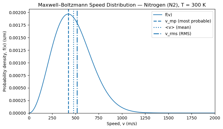
# Interactive plot: effect of temperature and molecular mass
#  * Temperature T shifts and broadens the distribution.
#  * Molecular mass m shifts the distribution:
#    heavier molecules have lower typical speeds at the same T.
#
# The plot shows f(v) vs. v and marks:
#  * v_mp: most probable speed (peak location)
#  * <v>: mean speed
#  * v_rms: root-mean-square speeds

# Checks at the end verify numerical calculations 
# ==============================================================================

# Generate a plot for Nitrogen at 300 K first; then make it interactive
def plot_mb(T=300.0, species="Nitrogen (N2)", v_max=2000, npts=2000, show_fills=False):
    M = species_db[species]               # g/mol
    m = molar_mass_to_molecule_mass(M)    # kg per molecule

    v = np.linspace(0, float(v_max), int(npts))
    f = f_MB(v, m, float(T))

    # characteristic speeds
    v_mp, v_mean, v_rms = speeds_characteristic(m, float(T))

    # numerical checks (integrals) — trapz is depricated. If you get an error, update numpy.
    area = np.trapezoid(f, v)  # should be ~1
    v_mean_num = np.trapezoid(v * f, v)
    v2_mean_num = np.trapezoid((v**2) * f, v)

    KE_avg_num = 0.5 * m * v2_mean_num  # J per molecule
    KE_avg_theory = 1.5 * kB * float(T)

    # Plot
    plt.figure(figsize=(8, 4.5))
    plt.plot(v, f)
    plt.axvline(v_mp, linestyle="--", linewidth=2)   # most probable
    plt.axvline(v_mean, linestyle=":", linewidth=2) # mean
    plt.axvline(v_rms, linestyle="-.", linewidth=2) # RMS


    plt.xlabel("Speed, v (m/s)")
    plt.ylabel("Probability density, f(v) (s/m)")
    plt.title(f"Maxwell–Boltzmann Speed Distribution — {species}, T = {T:.0f} K")
    plt.xlim(0, v_max)
    plt.ylim(bottom=0)

    if show_fills:
        mask = v <= v_mean
        plt.fill_between(v[mask], f[mask], alpha=0.2)

    plt.legend(
    ["f(v)",
     "v_mp (most probable)",
     "<v> (mean)",
     "v_rms (RMS)"],
    loc="upper right",
    frameon=True
  )

    plt.show()

    # --- IMPORTANT: this must be inside the function so area, etc. exist ---
    md = f"""### Numerical checks

- Normalization:  
  $\\int_0^\\infty f(v)\\,dv \\approx {area:.6f}$

- Mean speed:  
  numerical ${v_mean_num:.2f}\\,\\text{{m/s}}$,  
  theory ${v_mean:.2f}\\,\\text{{m/s}}$

- Mean squared speed:  
  numerical $\\langle v^2 \\rangle \\approx {v2_mean_num:.2e}\\,\\text{{(m/s)}}^2$,  
  theory ${(3*kB*float(T)/m):.2e}\\,\\text{{(m/s)}}^2$

### Average translational kinetic energy per molecule

- Numerical:  
$$
\\left\\langle \\tfrac{{1}}{{2}} m v^2 \\right\\rangle
\\approx {KE_avg_num:.3e}\\,\\text{{J}}
$$

- Theory:  
$$
\\tfrac{{3}}{{2}} k_B T
= {KE_avg_theory:.3e}\\,\\text{{J}}
$$
"""
    display(Markdown(md))


# Widgets + interactive output (unchanged)
T_slider = widgets.FloatSlider(value=300, min=50, max=2000, step=10,
                               description="T (K)", continuous_update=False)
species_dd = widgets.Dropdown(options=list(species_db.keys()),
                              value="Nitrogen (N2)",
                              description="Species")
vmax_slider = widgets.IntSlider(value=2000, min=500, max=6000, step=100,
                                description="v_max", continuous_update=False)
shade_toggle = widgets.Checkbox(value=False, description="Shade v ≤ <v>")

ui = widgets.VBox([
    widgets.HBox([T_slider, species_dd]),
    widgets.HBox([vmax_slider, shade_toggle])
])

out = widgets.interactive_output(
    plot_mb,
    {"T": T_slider, "species": species_dd, "v_max": vmax_slider, "show_fills": shade_toggle}
)

display(ui, out)

# Static preview: results for the default inputs above.
# The output is saved so the course website can show it.
# To try other inputs, use the controls above, or open
# this notebook in Colab (badge on the course website).
plot_mb(T=T_slider.value, species=species_dd.value,
        v_max=vmax_slider.value, show_fills=shade_toggle.value)

0.1 Numerical checks

Normalization:
\(\int_0^\infty f(v)\,dv \approx 1.000000\)
Mean speed:
numerical \(476.17\,\text{m/s}\),
theory \(476.17\,\text{m/s}\)
Mean squared speed:
numerical \(\langle v^2 \rangle \approx 2.67e+05\,\text{(m/s)}^2\),
theory \(2.67e+05\,\text{(m/s)}^2\)

0.2 Average translational kinetic energy per molecule

Numerical:
\[ \left\langle \tfrac{1}{2} m v^2 \right\rangle \approx 6.213e-21\,\text{J} \]
Theory:
\[ \tfrac{3}{2} k_B T = 6.213e-21\,\text{J} \]

Other Formats

0.1 Numerical checks

0.2 Average translational kinetic energy per molecule