# ===================================================================================================
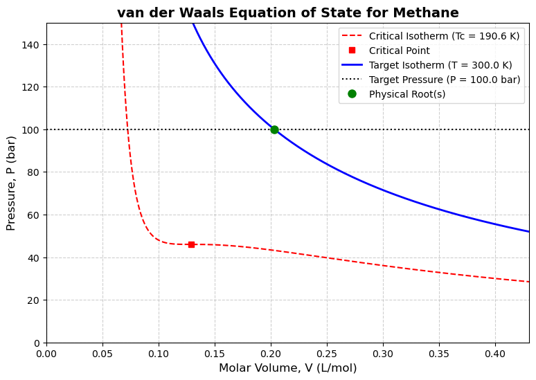
# LECTURE 27: Generalized van der Waals Equation of State Solver
# Author: Edward Maginn, CBE 20260
# Description:
#   This notebook solves the cubic van der Waals equation of state for a variety of
#   industrial gases. It fetches critical properties using CoolProp, converts user units,
#   solves for the molar volume roots, and plots the results on a P-V diagram.
# ===================================================================================================

# Install CoolProp if it is missing (e.g., on Google Colab)
try:
    import CoolProp
except ImportError:
    %pip install -q CoolProp

import numpy as np
import matplotlib.pyplot as plt
import ipywidgets as widgets
from IPython.display import display, clear_output
import CoolProp.CoolProp as CP

# Dictionary mapping friendly names to CoolProp string identifiers
fluid_dict = {
    'Methane': 'Methane',
    'Nitrogen': 'Nitrogen',
    'Oxygen': 'Oxygen',
    'Ethane': 'Ethane',
    'Ammonia': 'Ammonia',
    'Carbon Dioxide': 'CarbonDioxide',
    'Carbon Monoxide': 'CarbonMonoxide',
    'Argon': 'Argon',
    'Water': 'Water',
    'R-32': 'R32'
}

def solve_and_plot(fluid_name, T_val, T_unit, P_val, P_unit):
    fluid = fluid_dict[fluid_name]

    # --- 1. Unit Conversions to Standard Math Units (Kelvin & bar) ---
    if T_unit == '°C':
        T = T_val + 273.15
    elif T_unit == '°F':
        T = (T_val - 32) * 5/9 + 273.15
    else:
        T = T_val

    if P_unit == 'atm':
        P = P_val * 1.01325
    elif P_unit == 'Pa':
        P = P_val / 1e5
    elif P_unit == 'MPa':
        P = P_val * 10
    elif P_unit == 'psi':
        P = P_val / 14.5038
    else:
        P = P_val

    # Handle zero/negative T or P to prevent math errors
    if T <= 0 or P <= 0:
        print("Temperature and Pressure must be greater than absolute zero.")
        return

    # --- 2. Fetch Critical Properties ---
    Tc = CP.PropsSI('TCRIT', fluid)
    Pc_Pa = CP.PropsSI('PCRIT', fluid)
    Pc = Pc_Pa / 1e5  # Convert Pa to bar

    # --- 3. Calculate VDW Parameters ---
    R = 0.0831446 # L*bar/(mol*K)
    a = 27 * (R * Tc)**2 / (64 * Pc)
    b = R * Tc / (8 * Pc)

    # --- 4. Solve the Cubic Equation for Roots ---
    # V^3 - (b + RT/P)V^2 + (a/P)V - (ab/P) = 0
    C2 = -(b + R * T / P)
    C1 = a / P
    C0 = -a * b / P

    roots = np.roots([1, C2, C1, C0])

    # Filter out complex roots and non-physical roots (V < b)
    real_roots = roots[np.isclose(roots.imag, 0)].real
    real_roots = np.sort(real_roots[real_roots > b])

    # --- 5. Print Output Summary ---
    print("="*60)
    print(f"FLUID: {fluid_name}")
    print(f"Critical State: Tc = {Tc:.2f} K  |  Pc = {Pc:.2f} bar")
    print(f"VDW Parameters: a = {a:.4f} L^2·bar/mol^2  |  b = {b:.5f} L/mol")
    print("-" * 60)
    print(f"TARGET STATE:   T = {T:.2f} K  |  P = {P:.2f} bar")

    if len(real_roots) == 1:
        if T > Tc:
            state = "Supercritical Fluid"
        else:
            # Basic heuristic: if root is close to 'b', it's liquid, if close to ideal gas, it's vapor
            state = "Liquid" if real_roots[0] < 5*b else "Vapor"
        print(f"\n1 Real Root Found ({state}):")
        print(f"  ---> V = {real_roots[0]:.4f} L/mol")
    elif len(real_roots) == 3:
        print(f"\n3 Real Roots Found (Phase Split Region):")
        print(f"  ---> V_liquid   = {real_roots[0]:.4f} L/mol")
        print(f"  ---> V_unstable = {real_roots[1]:.4f} L/mol (non-physical)")
        print(f"  ---> V_vapor    = {real_roots[2]:.4f} L/mol")
    print("="*60)

    # --- 6. Plotting the P-V Diagram ---
    # Determine sensible bounds for the plot
    V_ig = R * T / P
    V_max = max(V_ig * 1.5, 10 * b)
    if len(real_roots) == 3:
        V_max = max(V_max, real_roots[2] * 1.3)

    V_arr = np.linspace(b * 1.02, V_max, 2000)

    # Calculate isotherms
    P_iso = (R * T) / (V_arr - b) - a / (V_arr**2)
    P_crit = (R * Tc) / (V_arr - b) - a / (V_arr**2)

    plt.figure(figsize=(9, 6))

    # Plot Critical Isotherm
    plt.plot(V_arr, P_crit, 'r--', lw=1.5, label=f'Critical Isotherm (Tc = {Tc:.1f} K)')
    plt.plot(3*b, Pc, 'rs', markersize=6, label='Critical Point')

    # Plot Selected Isotherm
    plt.plot(V_arr, P_iso, 'b-', lw=2, label=f'Target Isotherm (T = {T:.1f} K)')

    # Plot the Target Pressure line
    plt.axhline(P, color='k', linestyle=':', lw=1.5, label=f'Target Pressure (P = {P:.1f} bar)')

    # Plot roots
    for i, root in enumerate(real_roots):
        if len(real_roots) == 3 and i == 1:
            # Unstable root
            plt.plot(root, P, 'wo', markeredgecolor='k', markersize=8, label='Unstable Root' if i==1 else "")
        else:
            plt.plot(root, P, 'go', markersize=8, label='Physical Root(s)' if i==0 else "")

    # Formatting
    plt.ylim(0, max(P * 1.5, Pc * 1.5))
    plt.xlim(0, V_max)
    plt.xlabel('Molar Volume, V (L/mol)', fontsize=12)
    plt.ylabel('Pressure, P (bar)', fontsize=12)
    plt.title(f'van der Waals Equation of State for {fluid_name}', fontsize=14, fontweight='bold')
    plt.legend(loc='upper right')
    plt.grid(True, linestyle='--', alpha=0.6)

    plt.show()

# --- 7. Interactive UI Setup ---
style = {'description_width': 'initial'}

# Set default fluid to Methane
fluid_dropdown = widgets.Dropdown(options=list(fluid_dict.keys()), value='Methane', description='Fluid:')

# Set default Temperature to 300 K
T_input = widgets.FloatText(value=300, description='Temperature:', style=style, layout=widgets.Layout(width='200px'))
T_unit = widgets.Dropdown(options=['K', '°C', '°F'], value='K', layout=widgets.Layout(width='80px'))

# Set default Pressure to 100 bar
P_input = widgets.FloatText(value=100, description='Pressure:', style=style, layout=widgets.Layout(width='200px'))
P_unit = widgets.Dropdown(options=['bar', 'atm', 'Pa', 'MPa', 'psi'], value='bar', layout=widgets.Layout(width='80px'))

T_box = widgets.HBox([T_input, T_unit])
P_box = widgets.HBox([P_input, P_unit])

ui = widgets.VBox([fluid_dropdown, T_box, P_box])
out = widgets.interactive_output(solve_and_plot, {
    'fluid_name': fluid_dropdown,
    'T_val': T_input,
    'T_unit': T_unit,
    'P_val': P_input,
    'P_unit': P_unit
})

display(ui, out)