# Install CoolProp if it is missing (e.g., on Google Colab)
try:
    import CoolProp
except ImportError:
    %pip install -q CoolProp

import numpy as np
import matplotlib.pyplot as plt
import ipywidgets as widgets
from IPython.display import display, clear_output
import CoolProp.CoolProp as CP

# Dictionary mapping friendly names to CoolProp string identifiers
fluid_dict = {
    'Methane': 'Methane',
    'Nitrogen': 'Nitrogen',
    'Oxygen': 'Oxygen',
    'Ethane': 'Ethane',
    'Ammonia': 'Ammonia',
    'Carbon Dioxide': 'CarbonDioxide',
    'Carbon Monoxide': 'CarbonMonoxide',
    'Argon': 'Argon',
    'Water': 'Water',
    'R-32': 'R32'
}

def compute_residuals_and_plot(eos_choice, fluid_name, T_val, T_unit, P_val, P_unit):
    fluid = fluid_dict[fluid_name]

    # --- 1. Unit Conversions ---
    if T_unit == '°C': T = T_val + 273.15
    elif T_unit == '°F': T = (T_val - 32) * 5/9 + 273.15
    else: T = T_val

    if P_unit == 'atm': P = P_val * 1.01325
    elif P_unit == 'Pa': P = P_val / 1e5
    elif P_unit == 'MPa': P = P_val * 10
    elif P_unit == 'psi': P = P_val / 14.5038
    else: P = P_val

    if T <= 0 or P <= 0:
        print("Temperature and Pressure must be greater than zero.")
        return

    # --- 2. Fetch Critical Properties ---
    Tc = CP.PropsSI('TCRIT', fluid)
    Pc_Pa = CP.PropsSI('PCRIT', fluid)
    Pc = Pc_Pa / 1e5  # Convert Pa to bar
    omega = CP.PropsSI('ACENTRIC', fluid)

    # --- 3. Calculate EOS Parameters ---
    R_Lbar = 0.0831446 # L*bar/(mol*K)
    R_J = 8.31446      # J/(mol*K)
    Tr = T / Tc

    if eos_choice == 'SRK':
        ac = 0.42748 * (R_Lbar**2 * Tc**2) / Pc
        b = 0.08664 * R_Lbar * Tc / Pc
        m = 0.480 + 1.574 * omega - 0.176 * omega**2
    else: # Peng-Robinson
        ac = 0.45724 * (R_Lbar**2 * Tc**2) / Pc
        b = 0.07780 * R_Lbar * Tc / Pc
        m = 0.37464 + 1.54226 * omega - 0.26992 * omega**2

    alpha = (1 + m * (1 - np.sqrt(Tr)))**2
    a = ac * alpha
    da_dT = -ac * m * np.sqrt(alpha / (T * Tc))

    # --- 4. Solve the Cubic Equation ---
    C3 = 1.0
    if eos_choice == 'SRK':
        C2 = -(R_Lbar * T / P)
        C1 = (a / P) - b**2 - (R_Lbar * T * b / P)
        C0 = -(a * b / P)
    else: # Peng-Robinson
        C2 = b - (R_Lbar * T / P)
        C1 = (a / P) - 2 * b * (R_Lbar * T / P) - 3 * b**2
        C0 = b**3 + (R_Lbar * T / P) * b**2 - (a * b / P)

    roots = np.roots([C3, C2, C1, C0])
    real_roots = np.sort(roots[np.abs(roots.imag) < 1e-9].real)
    real_roots = real_roots[real_roots > b] # Must be physically greater than b

    # --- 5. Output Summary & Residuals ---
    print("="*70)
    print(f"SYSTEM: {fluid_name} modeled with {eos_choice} EOS")
    print(f"Critical State: Tc = {Tc:.2f} K  |  Pc = {Pc:.2f} bar  |  ω = {omega:.4f}")
    print(f"Parameters: a(T) = {a:.4f} L^2·bar/mol^2  |  b = {b:.5f} L/mol")
    print("-" * 70)
    print(f"TARGET STATE:   T = {T:.2f} K  |  P = {P:.2f} bar")

    V_ideal = R_Lbar * T / P
    print(f"Ideal Gas Vol:  V_ig = {V_ideal:.4f} L/mol")
    print("="*70)

    for i, root in enumerate(real_roots):
        if len(real_roots) == 1:
            phase = "Supercritical Gas" if T > Tc else ("Liquid" if root < 5*b else "Vapor")
        elif len(real_roots) == 3:
            if i == 0: phase = "Liquid Root"
            elif i == 1: phase = "Unstable Root (Non-Physical)"
            else: phase = "Vapor Root"

        print(f"\n[{phase}]")
        print(f"  Molar Volume (V) = {root:.4f} L/mol")

        if phase != "Unstable Root (Non-Physical)":
            V_R = root - V_ideal

            if eos_choice == 'SRK':
                log_term = np.log((root + b) / root)
                U_R = 100 * (T * da_dT - a) / b * log_term
                S_R = R_J * np.log(P * (root - b) / (R_Lbar * T)) + 100 * (da_dT / b) * log_term
            else: # Peng-Robinson
                log_term = np.log((root + (1 + np.sqrt(2))*b) / (root + (1 - np.sqrt(2))*b))
                U_R = 100 * (T * da_dT - a) / (2 * np.sqrt(2) * b) * log_term
                S_R = R_J * np.log(P * (root - b) / (R_Lbar * T)) + 100 * (da_dT / (2 * np.sqrt(2) * b)) * log_term

            H_R = U_R + 100 * P * V_R

            print(f"  Residual Volume   (V^R) = {V_R:.4f} L/mol")
            print(f"  Residual Internal (U^R) = {U_R:.1f} J/mol")
            print(f"  Residual Enthalpy (H^R) = {H_R:.1f} J/mol")
            print(f"  Residual Entropy  (S^R) = {S_R:.3f} J/(mol·K)")

    print("\n" + "="*70)

    # --- 6. Plotting the P-V Diagram ---
    V_max = max(V_ideal * 1.5, 10 * b)
    if len(real_roots) == 3:
        V_max = max(V_max, real_roots[2] * 1.3)

    V_arr = np.linspace(b * 1.05, V_max, 2000)

    if eos_choice == 'SRK':
        P_iso = (R_Lbar * T) / (V_arr - b) - a / (V_arr * (V_arr + b))
        alpha_c = (1 + m * (1 - 1))**2
        a_crit = ac * alpha_c
        P_crit = (R_Lbar * Tc) / (V_arr - b) - a_crit / (V_arr * (V_arr + b))
    else: # Peng-Robinson
        P_iso = (R_Lbar * T) / (V_arr - b) - a / (V_arr**2 + 2*b*V_arr - b**2)
        alpha_c = (1 + m * (1 - 1))**2
        a_crit = ac * alpha_c
        P_crit = (R_Lbar * Tc) / (V_arr - b) - a_crit / (V_arr**2 + 2*b*V_arr - b**2)

    plt.figure(figsize=(9, 6))
    plt.plot(V_arr, P_crit, 'r--', lw=1.5, label=f'Critical Isotherm (Tc = {Tc:.1f} K)')
    plt.plot(V_arr, P_iso, 'b-', lw=2, label=f'Target Isotherm (T = {T:.1f} K)')
    plt.axhline(P, color='k', linestyle=':', lw=1.5, label=f'Target Pressure (P = {P:.1f} bar)')

    for i, root in enumerate(real_roots):
        if len(real_roots) == 3 and i == 1:
            plt.plot(root, P, 'wo', markeredgecolor='k', markersize=8, label='Unstable Root' if i==1 else "")
        else:
            plt.plot(root, P, 'go', markersize=8, label='Physical Root(s)' if i==0 else "")

    plt.ylim(0, max(P * 1.5, Pc * 1.5))
    plt.xlim(0, V_max)
    plt.xlabel('Molar Volume, V (L/mol)', fontsize=12)
    plt.ylabel('Pressure, P (bar)', fontsize=12)
    plt.title(f'{eos_choice} Properties for {fluid_name}', fontsize=14, fontweight='bold')
    plt.legend(loc='upper right')
    plt.grid(True, linestyle='--', alpha=0.6)
    plt.show()

# --- 7. Interactive UI Setup ---
style = {'description_width': 'initial'}

eos_dropdown = widgets.Dropdown(options=['Peng-Robinson', 'SRK'], value='Peng-Robinson', description='EOS:', style=style)
fluid_dropdown = widgets.Dropdown(options=list(fluid_dict.keys()), value='Methane', description='Fluid:', style=style)

T_input = widgets.FloatText(value=300, description='Temperature:', style=style, layout=widgets.Layout(width='200px'))
T_unit = widgets.Dropdown(options=['K', '°C', '°F'], value='K', layout=widgets.Layout(width='80px'))

P_input = widgets.FloatText(value=100, description='Pressure:', style=style, layout=widgets.Layout(width='200px'))
P_unit = widgets.Dropdown(options=['bar', 'atm', 'Pa', 'MPa', 'psi'], value='bar', layout=widgets.Layout(width='80px'))

T_box = widgets.HBox([T_input, T_unit])
P_box = widgets.HBox([P_input, P_unit])

ui = widgets.VBox([eos_dropdown, fluid_dropdown, T_box, P_box])
out = widgets.interactive_output(compute_residuals_and_plot, {
    'eos_choice': eos_dropdown,
    'fluid_name': fluid_dropdown,
    'T_val': T_input,
    'T_unit': T_unit,
    'P_val': P_input,
    'P_unit': P_unit
})

display(ui, out)1 Advanced Cubic Equations of State and Residual Properties
Author: Edward Maginn, CBE 20260
In this notebook, we extend the residual property framework from the van der Waals equation to modern cubic equations of state: the Soave-Redlich-Kwong (SRK) and Peng-Robinson (PR) models. These models incorporate the acentric factor (\(\omega\)) and a temperature-dependent attractive parameter \(a(T)\), vastly improving their accuracy for real fluids, particularly near the vapor-liquid equilibrium region.
1.1 1. The Soave-Redlich-Kwong (SRK) Equation
The SRK equation improves upon the van der Waals model by modifying the attractive term in the denominator and making the parameter \(a\) dependent on temperature and the acentric factor: \[P = \frac{RT}{V - b} - \frac{a(T)}{V(V + b)}\]
The parameters are defined based on the critical properties: \[a_c = 0.42748 \frac{R^2 T_c^2}{P_c} \quad \text{and} \quad b = 0.08664 \frac{R T_c}{P_c}\] \[a(T) = a_c \alpha(T) \quad \text{where} \quad \alpha(T) = \left[1 + m\left(1 - \sqrt{\frac{T}{T_c}}\right)\right]^2\] \[m = 0.480 + 1.574 \omega - 0.176 \omega^2\]
To solve for the molar volume, the SRK equation is rearranged into a standard cubic polynomial in \(V\): \[V^3 - \left(\frac{RT}{P}\right)V^2 + \left(\frac{a}{P} - b^2 - \frac{RTb}{P}\right)V - \frac{ab}{P} = 0\]
1.1.1 SRK Residual Properties
By applying the fundamental thermodynamic property relations to the SRK equation, we can derive analytical expressions for the residual internal energy (\(U^R\)), residual enthalpy (\(H^R\)), and residual entropy (\(S^R\)): \[U^R = \frac{T \frac{da}{dT} - a}{b} \ln\left(\frac{V+b}{V}\right)\] \[H^R = U^R + P V^R\] \[S^R = R \ln\left(\frac{P(V-b)}{RT}\right) + \frac{1}{b} \frac{da}{dT} \ln\left(\frac{V+b}{V}\right)\]
1.2 2. The Peng-Robinson (PR) Equation
The Peng-Robinson equation further refines the volume dependence of the attractive term, which notably improves the prediction of liquid densities compared to SRK: \[P = \frac{RT}{V - b} - \frac{a(T)}{V(V + b) + b(V - b)}\]
The parameter definitions follow a similar structure but use different constants: \[a_c = 0.45724 \frac{R^2 T_c^2}{P_c} \quad \text{and} \quad b = 0.07780 \frac{R T_c}{P_c}\] \[m = 0.37464 + 1.54226 \omega - 0.26992 \omega^2\]
The standard cubic polynomial form for Peng-Robinson is: \[V^3 + \left(b - \frac{RT}{P}\right)V^2 + \left(\frac{a}{P} - \frac{2bRT}{P} - 3b^2\right)V + \left(b^3 + \frac{RTb^2}{P} - \frac{ab}{P}\right) = 0\]
1.2.1 Peng-Robinson Residual Properties
Because the denominator of the PR equation is more complex, the integral for the residual properties yields a slightly different logarithmic term: \[U^R = \frac{T \frac{da}{dT} - a}{2\sqrt{2}b} \ln\left(\frac{V+(1+\sqrt{2})b}{V+(1-\sqrt{2})b}\right)\] \[H^R = U^R + P V^R\] \[S^R = R \ln\left(\frac{P(V-b)}{RT}\right) + \frac{1}{2\sqrt{2}b} \frac{da}{dT} \ln\left(\frac{V+(1+\sqrt{2})b}{V+(1-\sqrt{2})b}\right)\]
1.3 Python Solver & Plotting Code
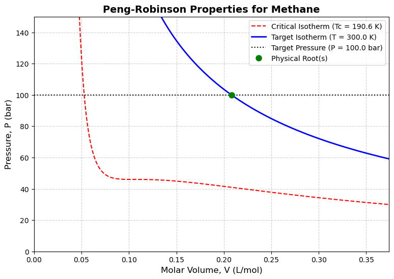
You can run this Python block to generate the interactive widgets, calculate the roots/residuals, and plot the isotherms.
# Static preview: results for the default inputs above.
# The output is saved so the course website can show it.
# To try other inputs, use the controls above, or open
# this notebook in Colab (badge on the course website).
compute_residuals_and_plot(eos_choice=eos_dropdown.value, fluid_name=fluid_dropdown.value,
                           T_val=T_input.value, T_unit=T_unit.value,
                           P_val=P_input.value, P_unit=P_unit.value)
======================================================================
SYSTEM: Methane modeled with Peng-Robinson EOS
Critical State: Tc = 190.56 K | Pc = 45.99 bar | ω = 0.0114
Parameters: a(T) = 2.0221 L^2·bar/mol^2 | b = 0.02680 L/mol
----------------------------------------------------------------------
TARGET STATE: T = 300.00 K | P = 100.00 bar
Ideal Gas Vol: V_ig = 0.2494 L/mol
======================================================================
[Supercritical Gas]
Molar Volume (V) = 0.2080 L/mol
Residual Volume (V^R) = -0.0414 L/mol
Residual Internal (U^R) = -1343.8 J/mol
Residual Enthalpy (H^R) = -1758.1 J/mol
Residual Entropy (S^R) = -4.241 J/(mol·K)
======================================================================