Lecture 24: Maxwell Relations
CBE 20260 / Thermodynamics I
1 Introduction: Using the Math of Thermodynamics
In the last lecture, we established that all thermodynamic state functions (\(U, H, A, G\)) have exact differentials. Using Legendre transforms, we showed that these expressions all contain the same information, just rearranged and written in terms of two different independent variables. We also introduced the Thermodynamic Square to help us remember these fundamental equations.
Today, we will use the properties of exact differentials to derive the Maxwell Relations. These relations are the “magic key” of thermodynamics. They allow us to take unmeasurable quantities like entropy derivatives and swap them for easily measurable \(P-V-T\) derivatives. By the end of this lecture, we will have rigorous equations to calculate \(\Delta S\), \(\Delta H\), and \(\Delta U\) for any real fluid from \(P-V-T\) data.
2 The Maxwell Relations
Last class, we showed that a state function \(F(x,y)\) has an exact differential of the form: \[dF = \left( \frac{\partial F}{\partial x} \right)_y dx + \left( \frac{\partial F}{\partial y} \right)_x dy \tag{1}\]
The partial derivatives in Eq. 1 are coefficients: \[dF = M(x,y) dx + N(x,y) dy\]
For example, our original fundamental equation for internal energy was: \[dU = T dS - P dV\]
The coefficients of the differentials are just the slopes of the surface in each direction: \[T = \left( \frac{\partial U}{\partial S} \right)_V \quad \text{and} \quad -P = \left( \frac{\partial U}{\partial V} \right)_S\]
Because thermodynamic variables are state functions, you can follow any path to calculate changes between equilibrium states. As shown in Fig. 1, you can follow constant \(S\) and \(V\) paths in any order to compute the change in \(U\); you don’t have to follow the “real” path. This is because \(U\), \(S\), and \(V\) are all state functions.
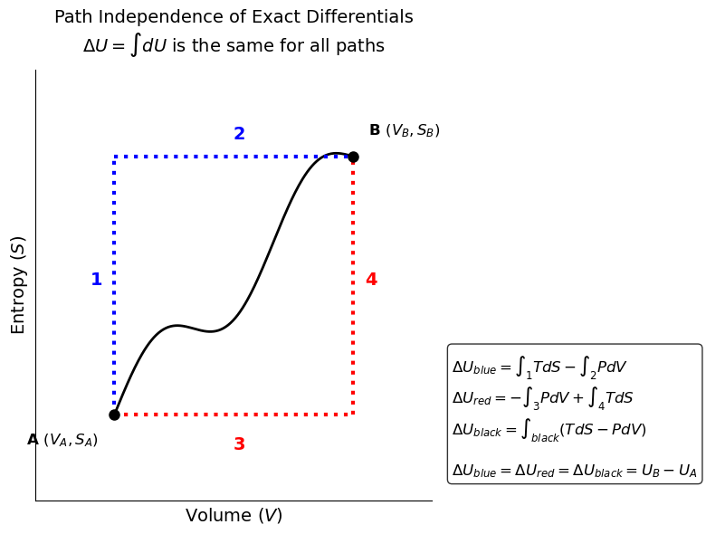
This has the following mathematical consequence. The order of differentiation does not matter for an exact differential. \[\left[ \frac{\partial}{\partial y} \left( \frac{\partial F}{\partial x} \right)_y \right ]_x = \left[ \frac{\partial}{\partial x} \left( \frac{\partial F}{\partial y} \right)_x \right ]_y\]
Referring to Eq. 1, if \(dF = M dx + N dy\), then the mixed second partial derivatives must be equal:
\[\left( \frac{\partial M}{\partial y} \right)_x = \left( \frac{\partial N}{\partial x} \right)_y \tag{2}\]
Let’s apply this rule systematically to the four fundamental equations.
2.1 From Internal Energy (\(U\))
\[dU = T dS - P dV\] Here, \(x = S, y = V, M = T, N = -P\). Applying the exactness criterion: \[\left( \frac{\partial T}{\partial V} \right)_S = -\left( \frac{\partial P}{\partial S} \right)_V \tag{3}\]
2.2 From Enthalpy (\(H\))
\[dH = T dS + V dP\] Applying the exactness criterion: \[\left( \frac{\partial T}{\partial P} \right)_S = \left( \frac{\partial V}{\partial S} \right)_P \tag{4}\]
2.3 From Helmholtz Free Energy (\(A\))
\[dA = -S dT - P dV\] Applying the exactness criterion: \[\left( \frac{\partial S}{\partial V} \right)_T = \left( \frac{\partial P}{\partial T} \right)_V \tag{5}\]
2.4 From Gibbs Free Energy (\(G\))
\[dG = -S dT + V dP\] Applying the exactness criterion: \[-\left( \frac{\partial S}{\partial P} \right)_T = \left( \frac{\partial V}{\partial T} \right)_P \tag{6}\]
Note: The last two Maxwell relations (from \(A\) and \(G\)) are by far the most useful in chemical engineering, because they relate entropy at a constant temperature directly to volumetric (\(P-V-T\)) properties.
Eq. 3 through Eq. 6 are the Maxwell Equations.
3 Calculating Entropy Changes
Let’s see the power of these relations in action. Suppose we want to calculate the change in entropy of a real gas, and we choose to use \(T\) and \(P\) as our independent variables. \[S = S(T, P)\]
Taking the total differential: \[dS = \left( \frac{\partial S}{\partial T} \right)_P dT + \left( \frac{\partial S}{\partial P} \right)_T dP\]
We need to replace these two partial derivatives with measurable quantities.
The Temperature Derivative: Recall the definition of constant-pressure heat capacity: \(C_p = \left( \frac{\partial H}{\partial T} \right)_P\). Since \(dH = T dS + V dP\), at constant pressure (\(dP = 0\)), \(dH = T dS\). Therefore: \[C_p = T \left( \frac{\partial S}{\partial T} \right)_P \implies \left( \frac{\partial S}{\partial T} \right)_P = \frac{C_p}{T}\]
The Pressure Derivative: We apply the Maxwell relation from the Gibbs Free Energy (Eq. 6): \[\left( \frac{\partial S}{\partial P} \right)_T = -\left( \frac{\partial V}{\partial T} \right)_P\]
Substitute these back into the total differential: \[dS(T, P) = \frac{C_p}{T} dT - \left( \frac{\partial V}{\partial T} \right)_P dP \tag{7}\]
If we instead chose \(T\) and \(V\) as our variables, \(S = S(T,V)\), we would use \(C_v\) and the Maxwell relation from \(A\) to get: \[dS(T, V) = \frac{C_v}{T} dT + \left( \frac{\partial P}{\partial T} \right)_V dV \tag{8}\]
Remember we derived an expression for the change in entropy of an ideal gas in terms of \(T\) and \(P\): \[\Delta S = C_p \ln \left( \frac{T_2}{T_1} \right) - R \ln \left( \frac{P_2}{P_1} \right)\] This is just the integrated form of Eq. 7 for an ideal gas, where \(\left( \frac{\partial V}{\partial T} \right)_P = \frac{R}{P}\). For a real gas, that term is not \(\frac{R}{P}\), and the change in entropy is more complicated. However, Eq. 7 is still exact and can be used to calculate the change in entropy of any real fluid from \(P-V-T\) data!
The same is true for the change in entropy of a real fluid as a function of \(T\) and \(V\) using Eq. 8. For an ideal gas, \(\left( \frac{\partial P}{\partial T} \right)_V = \frac{R}{V}\), and we recover the ideal gas expression for \(\Delta S\) in terms of \(T\) and \(V\). For a real fluid, that term is not \(\frac{R}{V}\), but Eq. 8 still holds and can be used to calculate the change in entropy from \(P-V-T\) data.
.