# ==============================================================================
# LECTURE 19: Regenerative Rankine Cycle
# Script: rankine-regen.ipynb
# Author: Edward Maginn, CBE 20260
# Description:
# This notebook performs a thermodynamic analysis of a regenerative Rankine
# cycle with one open feedwater heater (OFWH). It calculates the states, work,
# heat, and thermal efficiency of the cycle based on user inputs for boiler
# pressure, boiler temperature, extraction pressure, condenser pressure,
# and isentropic efficiency. The notebook uses CoolProp to obtain fluid
# properties and ipywidgets to create an interactive interface for exploring
# how different operating conditions affect cycle performance.
# ==============================================================================

# Install CoolProp if it is missing (e.g., on Google Colab)
try:
    import CoolProp
except ImportError:
    %pip install -q CoolProp

import CoolProp.CoolProp as CP
import ipywidgets as widgets
from IPython.display import display, clear_output

def solve_regenerative_rankine(P_boiler_bar, T_boiler_C, P_extract_bar, P_cond_bar, eta):
    """
    Calculates the states and efficiency of a Regenerative Rankine Cycle
    with one Open Feedwater Heater (OFWH). Uses IUPAC sign convention.
    """
    fluid = 'Water'

    # Check for non-physical pressure selections from sliders
    if P_extract_bar >= P_boiler_bar or P_extract_bar <= P_cond_bar:
        print("Error: Extraction pressure must be between Boiler and Condenser pressures.")
        return

    # Convert pressures to Pa and Temp to K for CoolProp
    P1 = P_boiler_bar * 1e5
    T1 = T_boiler_C + 273.15
    P_ex = P_extract_bar * 1e5
    P_cond = P_cond_bar * 1e5

    try:
        # --- STEP 1: Boiler Out / HP Turbine In (State 5) ---
        # Properties come from CoolProp calls
        H1 = CP.PropsSI('H', 'P', P1, 'T', T1, fluid) / 1000  # kJ/kg
        S1 = CP.PropsSI('S', 'P', P1, 'T', T1, fluid) / 1000  # kJ/kg-K

        # --- STEP 2: HP Turbine Out / Extraction (State 2) ---
        # Ideal
        S2_ideal = S1
        H2_ideal = CP.PropsSI('H', 'P', P_ex, 'S', S2_ideal * 1000, fluid) / 1000
        W_HP_rev = H2_ideal - H1 # IUPAC: Negative
        # Actual
        W_HP = W_HP_rev * eta
        H2 = H1 + W_HP
        S2_actual = CP.PropsSI('S', 'P', P_ex, 'H', H2 * 1000, fluid) / 1000

        # --- STEP 3: LP Turbine Out / Condenser In (State 3) ---
        # Ideal
        S3_ideal = S2_actual
        H3_ideal = CP.PropsSI('H', 'P', P_cond, 'S', S3_ideal * 1000, fluid) / 1000
        W_LP_rev = H3_ideal - H2 # IUPAC: Negative
        # Actual
        W_LP = W_LP_rev * eta
        H3 = H2 + W_LP

        # --- STEP 4: Condenser Out / Pump 1 In (State 4) ---
        H4 = CP.PropsSI('H', 'P', P_cond, 'Q', 0, fluid) / 1000 # Sat Liquid
        D4 = CP.PropsSI('D', 'P', P_cond, 'Q', 0, fluid) # kg/m^3
        V4 = 1 / D4 # m^3/kg

        # --- STEP 5: Pump 1 Out / OFWH In (State 5) ---
        W_P1_rev = V4 * (P_ex - P_cond) / 1000 # kJ/kg. IUPAC: Positive
        W_P1 = W_P1_rev / eta
        H5 = H4 + W_P1

        # --- STEP 6: OFWH Out / Pump 2 In (State 6) ---
        H6 = CP.PropsSI('H', 'P', P_ex, 'Q', 0, fluid) / 1000 # Sat Liquid
        D6 = CP.PropsSI('D', 'P', P_ex, 'Q', 0, fluid)
        V6 = 1 / D6

        # --- MASS BALANCE: Open Feedwater Heater ---
        # y*H2 + (1-y)*H5 = H6
        y = (H6 - H5) / (H2 - H5)

        # --- STEP 7: Pump 2 Out / Boiler In (State 7) ---
        W_P2_rev = V6 * (P1 - P_ex) / 1000 # kJ/kg
        W_P2 = W_P2_rev / eta
        H7 = H6 + W_P2

        # --- CYCLE PERFORMANCE ---
        W_turb_total = W_HP + (1 - y) * W_LP
        W_pump_total = (1 - y) * W_P1 + W_P2
        W_net = W_turb_total + W_pump_total

        Q_H = H1 - H7

        thermal_efficiency = -W_net / Q_H

        # --- PRINT RESULTS ---
        print("-" * 50)
        print(f"REGENERATIVE RANKINE CYCLE ANALYSIS")
        print("-" * 50)
        print(f"Extraction Fraction (y):     {y:.4f}  ({y*100:.1f}%)")
        print("-" * 50)
        print(f"HP Turbine Work (per kg):    {W_HP:.2f} kJ/kg")
        print(f"LP Turbine Work (per kg):    {W_LP:.2f} kJ/kg")
        print(f"Total Turbine Work:          {W_turb_total:.2f} kJ/kg")
        print(f"Total Pump Work:             {W_pump_total:.2f} kJ/kg")
        print(f"Net Work (W_net):            {W_net:.2f} kJ/kg")
        print(f"Heat Added (Q_H):            {Q_H:.2f} kJ/kg")
        print("-" * 50)
        print(f"THERMAL EFFICIENCY:          {thermal_efficiency*100:.2f} %")
        print("-" * 50)

    except Exception as e:
        print(f"Fluid property error. Trying to calculate outside valid region. ({e})")

# --- CREATE INTERACTIVE WIDGETS TO INPUT OPERATING PARAMETERS ---
style = {'description_width': 'initial'}

slider_P_boiler = widgets.FloatSlider(value=60.0, min=20.0, max=150.0, step=1.0, description='Boiler Pressure (bar):', style=style)
slider_T_boiler = widgets.FloatSlider(value=500.0, min=300.0, max=600.0, step=5.0, description='Boiler Temp (°C):', style=style)
slider_P_extract = widgets.FloatSlider(value=10.0, min=2.0, max=30.0, step=1.0, description='Extraction Pressure (bar):', style=style)
slider_P_cond = widgets.FloatSlider(value=1.0, min=0.05, max=2.0, step=0.05, description='Condenser Pressure (bar):', style=style)
slider_eta = widgets.FloatSlider(value=0.75, min=0.5, max=1.0, step=0.01, description='Isentropic Efficiency (η):', style=style)

# Group them into a nice vertical layout
ui = widgets.VBox([slider_P_boiler, slider_T_boiler, slider_P_extract, slider_P_cond, slider_eta])

# Define the output display connection
out = widgets.interactive_output(solve_regenerative_rankine, {
    'P_boiler_bar': slider_P_boiler,
    'T_boiler_C': slider_T_boiler,
    'P_extract_bar': slider_P_extract,
    'P_cond_bar': slider_P_cond,
    'eta': slider_eta
})

# Display the interface
display(ui, out)
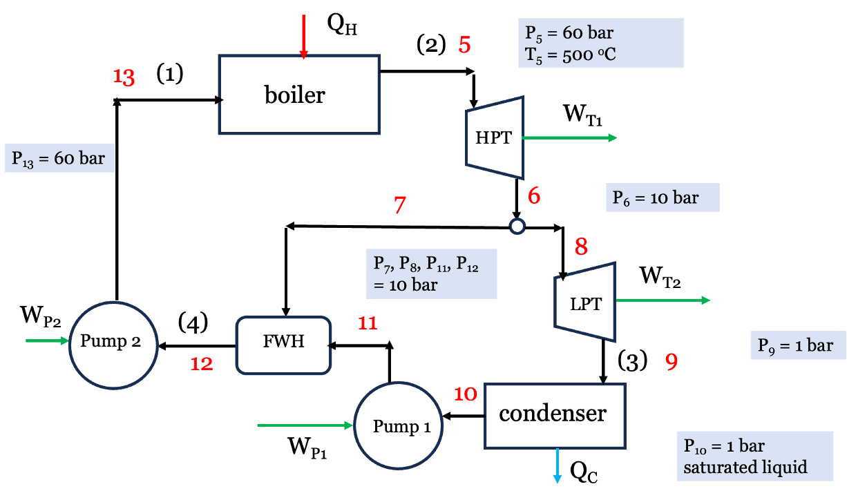
Figure 1. Modified Rankine Cycle with open feedwater heater.
# Static preview: results for the default inputs above.
# The output is saved so the course website can show it.
# To try other inputs, use the controls above, or open
# this notebook in Colab (badge on the course website).
solve_regenerative_rankine(P_boiler_bar=slider_P_boiler.value, T_boiler_C=slider_T_boiler.value,
                           P_extract_bar=slider_P_extract.value, P_cond_bar=slider_P_cond.value,
                           eta=slider_eta.value)
--------------------------------------------------
REGENERATIVE RANKINE CYCLE ANALYSIS
--------------------------------------------------
Extraction Fraction (y): 0.1308 (13.1%)
--------------------------------------------------
HP Turbine Work (per kg): -377.03 kJ/kg
LP Turbine Work (per kg): -346.55 kJ/kg
Total Turbine Work: -678.24 kJ/kg
Total Pump Work: 8.60 kJ/kg
Net Work (W_net): -669.63 kJ/kg
Heat Added (Q_H): 2653.08 kJ/kg
--------------------------------------------------
THERMAL EFFICIENCY: 25.24 %
--------------------------------------------------