vdw-tp – CBE 20260 — Course Notes

# ===================================================================================================
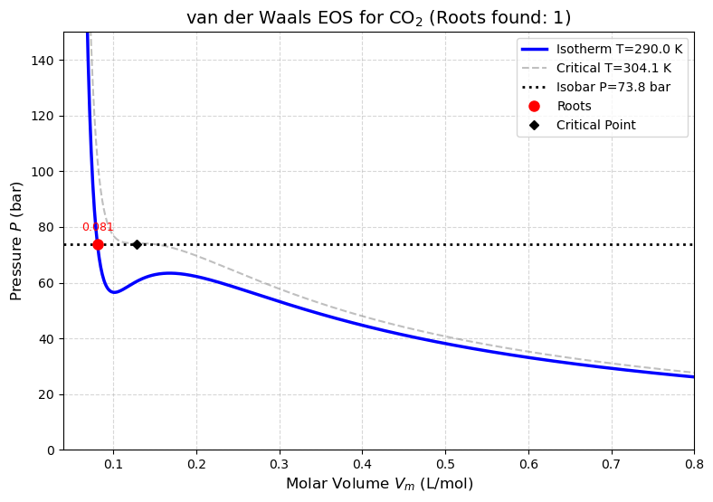
# LECTURE 7: VDW EOS solver showing solutions for T and P
# Script: VDW-TP
# Author: Edward Maginn, CBE 20260
# Description: 
#   This notebook visualizes the van der Waals equation of state for CO2. It allows 
#   users to interactively change temperature and pressure to see how many real 
#   volume roots exist for the given conditions.
#   The van der Waals parameters for CO2 are used, and the critical point is highlighted.
# ====================================================================================
# On Google Colab, install ipympl and enable interactive widgets
import sys
if "google.colab" in sys.modules:
    %pip install -q ipympl
    from google.colab import output
    output.enable_custom_widget_manager()

import numpy as np
import matplotlib.pyplot as plt
from ipywidgets import interact, FloatSlider

# Constants for CO2
a_CO2 = 3.64  # L^2 bar mol^-2
b_CO2 = 0.04267 # L mol^-1
Tc_CO2 = 304.13 # K
Pc_CO2 = 73.77  # bar
R = 0.08314  # L*bar/(mol*K)

def vdw_pressure(T, V_m, a, b):
    return (R * T) / (V_m - b) - a / (V_m**2)

def solve_vdw_roots(P, T, a, b):
    """
    Finds real volume roots for vdW equation at given P and T.
    Rearranged cubic form: P*V^3 - (Pb + RT)*V^2 + a*V - ab = 0
    """
    # Coefficients for cubic polynomial: c3*V^3 + c2*V^2 + c1*V + c0 = 0
    c3 = P
    c2 = -(P * b + R * T)
    c1 = a
    c0 = -a * b
    
    roots = np.roots([c3, c2, c1, c0])
    
    # Filter for real roots that are physically meaningful (V > b)
    valid_roots = [r.real for r in roots if np.isreal(r) and r.real > b]
    return np.sort(valid_roots)

def plot_vdw_simulation(T, P_user):
    
    # 1. Setup Plot
    v = np.linspace(b_CO2 * 1.1, 1.0, 1000)
    P_curve = vdw_pressure(T, v, a_CO2, b_CO2)
    
    fig, ax = plt.subplots(figsize=(9, 6))
    
    # 2. Plot the Isotherm (Blue Curve)
    ax.plot(v, P_curve, linewidth=2.5, color='blue', label=f'Isotherm T={T:.1f} K')
    
    # 3. Plot the Critical Isotherm (Gray Dashed)
    P_crit = vdw_pressure(Tc_CO2, v, a_CO2, b_CO2)
    ax.plot(v, P_crit, '--', color='gray', alpha=0.5, label=f'Critical T={Tc_CO2:.1f} K')
    
    # 4. Plot the User's Isobar (Horizontal Line)
    ax.axhline(P_user, color='black', linestyle=':', linewidth=2, label=f'Isobar P={P_user:.1f} bar')
    
    # 5. Find and Plot Intersections
    roots = solve_vdw_roots(P_user, T, a_CO2, b_CO2)
    
    # Plot the roots
    for i, vol in enumerate(roots):
        label = "Roots" if i == 0 else "_nolegend_"
        ax.plot(vol, P_user, 'ro', markersize=8, zorder=5, label=label)
        # Annotate the volume values
        ax.text(vol, P_user + 5, f'{vol:.3f}', horizontalalignment='center', color='red', fontsize=9)

    # 6. Formatting
    ax.set_ylim(0, 150)
    ax.set_xlim(0.04, 0.8)
    # Using V_m to avoid LaTeX error with \underline
    ax.set_xlabel('Molar Volume $V_m$ (L/mol)', fontsize=12)
    ax.set_ylabel('Pressure $P$ (bar)', fontsize=12)
    ax.set_title(f'van der Waals EOS for CO$_2$ (Roots found: {len(roots)})', fontsize=14)
    
    # Highlight Critical Point
    ax.plot(3*b_CO2, Pc_CO2, 'kD', markersize=5, label='Critical Point')
    
    ax.legend(loc='upper right')
    ax.grid(True, linestyle='--', alpha=0.5)
    plt.show()

# Interactive Slider
# T: 250K to 350K
# P: 10 bar to 120 bar
interact(plot_vdw_simulation, 
         T=FloatSlider(value=290, min=250, max=350, step=1.0, description='Temp (K)'),
         P_user=FloatSlider(value=Pc_CO2, min=10, max=120, step=1.0, description='Press (bar)'));

Running locally.

# Static preview: results for the default inputs above.
# The output is saved so the course website can show it.
# To try other inputs, use the controls above, or open
# this notebook in Colab (badge on the course website).
plot_vdw_simulation(T=290, P_user=Pc_CO2)

Other Formats